About

Recently I’ve been playing about with a STM32F4DISCOVERY project which requires some DSP - nothing special, just a low pass filter. My DSP is pretty rusty however, and it probably could have been described that way even when I was studying it in uni. I was always able to recall the various formula and when to use them, but the fundamental understanding of just what the math was doing never materialised.

So when I found myself requiring to implement a low pass filter “in real life”, and not as a question on some test paper or coursework, I done what any sane person would do. I dusted off the text book went looking for suitable libraries I could use. After a brief search, I decided that the FIR functions offered in ARM’s CMSIS package seemed like a pretty solid bet.

As part of the CMSIS library, ARM offers several different FIR filtering functions. Some versions operate on different datatypes while others are “fast” variants; typically sacrificing some accuracy for speed. Being curious about this plethora of FIR filtering functions and how they perform, I put together a crude test to compare them. The results of this can be seen below.

Test

All the code I used can be found in this github repository, at the tag TEST_CMSIS_FIR_1. If you are interested in reproducing the test, I have included some basic instructions on how to do this. They can be found in test/cmsis_fir_filters/README.md.

An overview of the process is as follows:

1. The file test/cmsis_fir_filters/utils/design.py is responsible for creating the C files containing FIR filter coefficients and a test signal. Additionally it computes the expected filtered signal.

2. The output coefficients and test signal are to be compiled along with the rest of test/cmsis_fir_filters/src/, flashed to the MCU and executed. The filtered output from the CMSIS arm_fir_*() functions and timing data can be retrieved with GDB.

   I was somewhat curious to see how well GCC optimised the CMSIS functions, so this step is repeated twice, once with a binary compiled with the option -O0 and again with -O2.

3. The second Python script, test/cmsis_fir_filters/utils/compare.py parses the output from GDB and test/cmsis_fir_filters/utils/design.py. Using this information, it graphs the deviation between expected and calculated filtered signals as well as the CPU cycles consumed by the filtering functions.

Signal

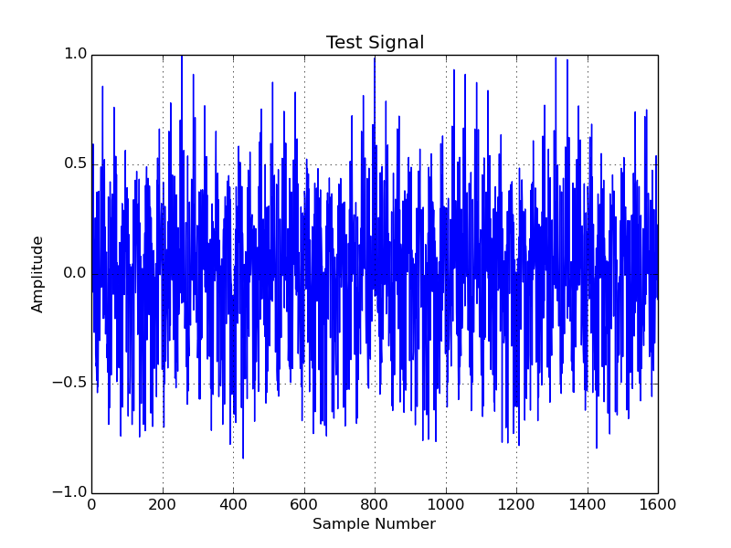
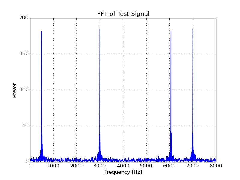
The generated test signal to be filtered is 100 ms (1600 samples) of a 16 kHz signal. It consists of 4 individual sinusoids as well as a small amount of noise, which has been thrown in for good measure. If anyone is curious, the signal and it’s FFT can be seen below.

FIR Design

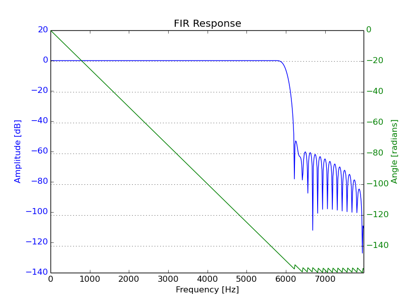
The FIR filter is a 128 tap (127 order) filter, intended to produce a cut-off frequency at 6 kHz for a sampling frequency of 16 kHz.

A graph of the filter’s response can be seen below.

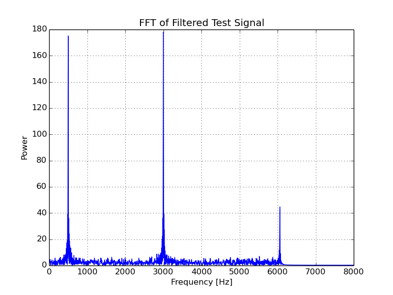
In the next graph, you can see the anticipated effect of filtering the test signal through this.

Results

Time

The CMSIS FIR functions are designed to work on continuous data (as opposed to the single call of scipy.signal.lfilter() in design.py). They require an argument containing an array (“block”) of newly acquired samples to be processed. The 100 ms test sample was (somewhat arbitrarily) divided up into 25, 64-sample blocks for processing. This equates to one block being provided to the CPU every 4 ms. During this test, the STM32F407 was being operated at its maximum clock speed of 168 MHz, in which case 4 ms is the equivalent of 672000 clock cycles.

If filtering the signal was the only processing required, this value would be the hard limit on the number of cycles available to filter one block of samples. The actual limit will be significantly less than this; varying with the program’s intended application. Typically the signal will have been filtered for some purpose, so extra overhead will exist in the form of additional signal processing or communication with another device, etc.

ChibiOS’s Time Measurement functionality was used to measure the (approximate) number of cycles required by the filtering functions to process a block of data. On the STM32F4 this value is retrieved from the DWT unit’s CYCCNT register, so hopefully should be pretty accurate.

The table below shows the measured cycles per block calculation, and the equivalent percentage load this had on the CPU.

Filter	Unoptimised (-O0) Cycles	Unoptimised (-O0) Load (%)	Optimised (-O2) Cycles	Optimised (-O2) Load (%)
Q15	256424	38.2	83846	12.5
Q15 Fast	155267	23.1	14382	2.1
Q31	386913	57.6	33838	5.0
Q31 Fast	239335	35.6	81469	12.1
Float	135114	20.1	28862	4.3

Same results, but a little prettier:

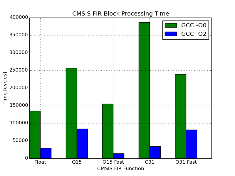
Some observations on these results:

• GCC does a pretty good job of optimising across the board. There is a notable performance increase for all the filtering functions. This varies between an approximate 3x improvement for the Q31 Fast function and a 11x improvement for Q31.

• After optimisation the Q31 Fast function performs slower than than the “normal” Q31 function. I haven’t delved into the compiled assembly to try and find the reason for this. I would be tempted to put this down to a quirk in GCC, or perhaps more likely, an error on my part. At the time of writing I am happy to treat the compiler as a black box rather than attempt to make sense of how it has optimised these functions.

  I did attempt Googling for similar CMSIS benchmarks, but the only similar post I found was this, which lists detailed FIR benchmarks against a Freescale K70. Freescale forum user Poul-Erik Hansen’s results do not match my own. They show that for more than one sample Q31 Fast outperforms Q31. He used IAR rather than GCC as the compiler, and there is no mention of some form of optimisation being enabled (but I assume it would be).

• The hardware floating point calculations are fast. Unoptimised, they outperform all other unoptimised functions. Considering only the optimised results, Q15 Fast is the only function to process a block faster.

Accuracy

As mentioned above, the Python script not only produced the filter coefficients but also calculated the “expected” filtered signal. This was then compared against each output of the various CMSIS functions.

These measurements should be taken with a pinch of salt since floating point numbers were being passed around in string form and I couldn’t find how to tweak GDB’s floating point representation. In hindsight I probably should have considered passing about the hexadecimal variants, but then of course I would have had to worry about the conversion back to float.

To compare the accuracy of the results, I picked two simple metrics:

• Max Sample Deviation - The greatest difference between samples, when comparing each individual sample of the CMSIS calculated signal against the one generated by Python.
• Root Mean Square Deviation - A slightly more rigorous measure, calculated by considering the deviation of all samples.

These two measurements can be seen in the graphs below for each filter. Note that the scale is logarithmic to ensure that Q15 results can exist on the same scale as the other functions. As you would expect, the Q15 functions suffer greatly from only having half the number of bits available to store the samples.

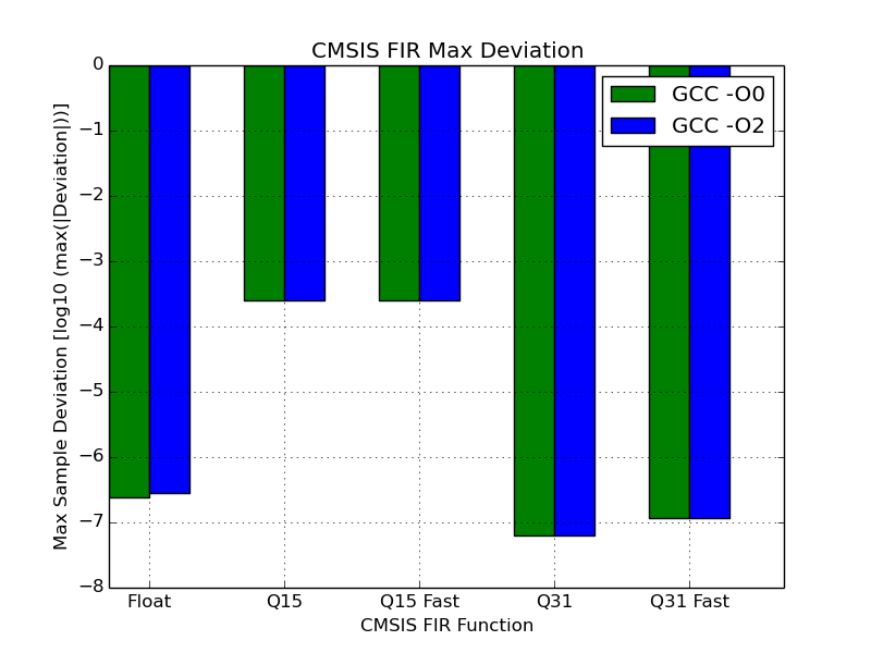
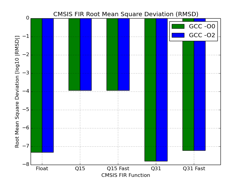
Below is a table with the results. For all but float, the calculated output was unchanged with optimisation so the results have not been duplicated.

Filter	Max Deviation (-O0)	Root Mean Square Deviation (-O0)
Q15	0.000246477676267	0.000115541718721
Q15 Fast	0.000246477676267	0.000115541718721
Q31	6.42909881998e-08	1.59465738538e-08
Q31 Fast	1.16589762678e-07	6.04082295228e-08
Float	2.39170974359e-07	4.87415531383e-08

Filter	Max Deviation (-O2)	Root Mean Square Deviation (-O2)
Float	2.86760586443e-07	4.83186829429e-08

Some observations:

• The filtered signal output of the floating point functions unexpectedly varied with GCC optimisation level. The maximum deviation of the samples in the floating point signal can be observed to be larger when the optimised function is used. However, the RMSD of the optimised function’s output is actually slightly lower, thus the signal as a whole is closer to the one expected.

  I briefly investigated this and through some trial and error found:

  • optimising using either -O1 or-Og resulted in no difference in the optimised and unoptimised floating point output signals.
  • optimising with either -Os or -O2 resulted in the optimised and unoptimised functions producing different outputs.

  Going slightly deeper down the rabbit hole it was observed that:

  • with the optimisation level set to -O2 and disabling expensive optimisations with -fno-expensive-optimizations the optimised and unoptimised floating point functions produced the same result.
  • enabling expensive optimisations with -fexpensive-optimizations along with -O1 did not cause any change in the output of the floating point functions.

  It appears as though this behaviour is due to interaction between several optimisation options. I did not attempt to narrow it down any further than this. It should be noted that since I attempted this test with the one set of inputs, it is quite possible this is simply an anomaly.

• For this sample, the Q31 variant produces an output that is closer to the expected signal than the floating point variant. This suggests that the magnitude of the output was close enough to that of the input signal that the benefit of having a floating point didn’t come into play.

Thoughts

I originally attempted to design the filter in Octave, which is essentially a Matlab clone. However, it wasn’t long before the many reasons why I disliked using Matlab came flooding back. This lead me to change camps to the Python SciPy/NumPy/matplotlib alternative, which I will happily recommend to anyone doing something similar.

For my future project, I’ve settled on using the floating point function, arm_fir_f32(). With the floating point hardware on the STM32F407 enabling fast and accurate floating point calculations I think I would be silly not to. It’s noted that the Q31 functions could squeeze out an extra drop of precision at the cost of only a few cycles. In my use case however I can afford to sacrifice some precision in order to avoid using datatypes non-native to C.

This was the first time I’ve dabbled with fixed point calculations in C and will admit to finding them fairly off-putting. If you are looking for somewhere to start I found Fixed Point Arithmetic on the ARM to be short, sweet and to the point on the matter. This wasn’t the only document I consulted, but its presentation of the maths helped tie everything else I read together.

Dependencies

Package	Version	Source
ChibiOS	20cb09025dc2884dd3269ac889c4ac2a5c74c93b	https://github.com/ChibiOS/ChibiOS
CMSIS	8c0e1a91341cde86532b05625f2ad584ce856118	https://github.com/ARM-software/CMSIS
gcc-arm-none-eabi	4.8.3-11ubuntu1+11	old-releases.ubuntu.com/ubuntu/ utopic/universe amd64 Packages